Introduction
Hello it's a me again Drifter Programming!
Today we continue with Electromagnetism to get into Equipotential surfaces and potential gradient!
I highly suggest you to read my previous posts of this series to understand potential energy and potential and even get back to electric fields and field lines cause what we will get into today will seem similar to electric field lines!
So, without further do, let's dive straight into it!
Equipotential surface
Electric field lines (that we talked about previously) help us understand electric fields, cause they give us an "visual" representation of an Electric field! Each of those lines represents the "direction" of the electric field, cause the electric field (vector) is tangent to each point of those lines!
In a similar way, the potential at points inside of an electric field can be represented "graphically" using Equipotential surfaces!
An Equipotential surface is a surface where the potential is the same (equal) for any point on top of that surface.
In an area where an electric field exists we can construct an equipotential surface that passes through any point. In the diagrams we only show some equipotential lines, mostly with the same potential difference between neighbouring surfaces. And lasty, no point can have 2 or more different potentials and so equipotential lines can never be tangent and can never intersect!
But, why do we need those surfaces?
Well, when moving "along" an equipotential surface the potential is the same for any point where an test charge passes by. Which means that the electric field E doesn't produce Work to the test charge on top of an equipotential surface! More specifically the electric field E can't have an vector component tangent to that surface, so that this component can produce Work to the motion of the moving charge on top of the surface.
So, the electric field is vertically across to any point of the equipotential surface and to the equipotential surface as a whole! Something which gets us to the conclusion that:
Electric field lines and Equipotential surfaces are always vertically across to each other!
Generally, electric field lines are curved lines and equipotential surfaces are curved surfaces. In the special case of an uniform field where the electric field lines are parallel to each other, the equipotential surfaces are parallel surfaces vertically across to the electric field's lines.
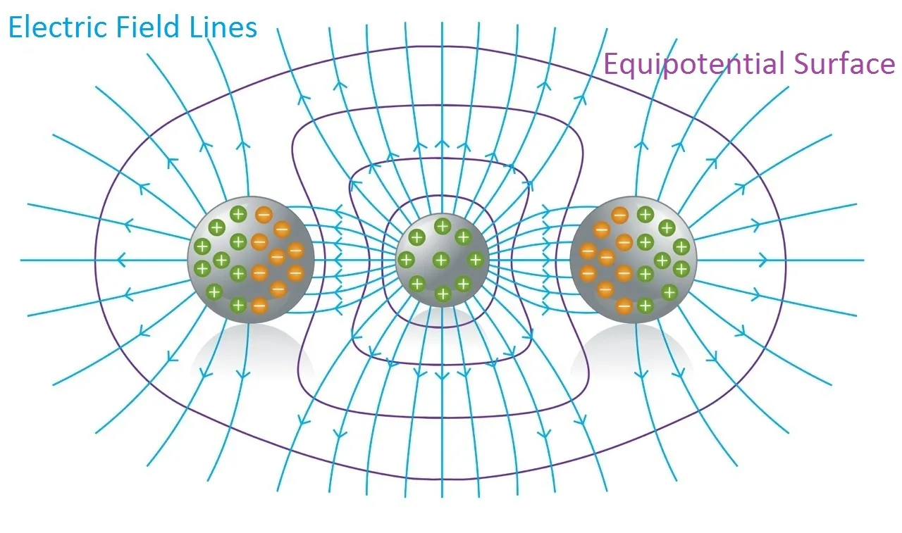
Here you can see some arrangements of charges:
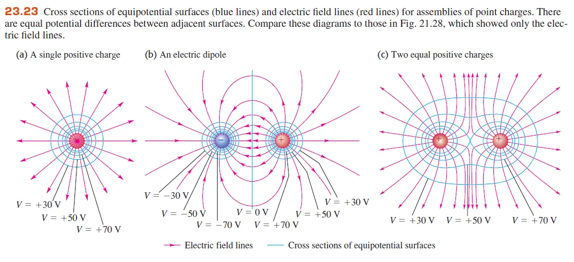
- The red lines are the electric field lines
- The blue lines are the equipotential surfaces
Of course the electric field, field lines and equipotential surfaces are actually 3-dimensional, but either way you can still see that the equipotential "lines" vertically intersect with the electric field's lines!
Something worth noting is:
When the charges inside of a conductor are not moving (are at "rest") then the electric field directly outside of the conductor must be vertically across to every point on top of it's surface.
Of course the electric field E = 0 in every point inside of the conductor (electrostatics), cause else the charges would be moving! This means that the component of E that is tangent to the surface, inside of the conductor, is zero at every point. Therefore the tangent component of E directly outside of the conductor is also zero. If that was not true then we would violate the laws of electrostatics. And so, the electric field is vertically across to every point of the conductor's surface.
As a result:
An conductive surface is always an equipotential surface!
Let's now get into something "mathematical"...
Potential Gradient
We know that the electric field and potential are tightly connected to each other.
You might remember the following equation from last time:

So, when knowing the electric field E at different points then we can use this equation to calculate potential differences. We can of course also do the opposite and determine the electric field E by knowing the potential V at different points.
Let's assume that the potential V is a function of the coordinates (x, y, z) that represent a point in Cartesian space. Let's find out if the electric field E (or it's components) will again be closely binded to V and in which way.
Last time we said that the potential difference between two points a and b can also be noted as:

This of course describes the change of potential when moving from point b to point a!
Using a very small (infinitesimal) change dV of potential that describes the change of potential when moving a very small distance dl we can write the following:

Let's also assume the parallel to dl component of E.
Using this component we can rewrite the first equation as:

And so, these two integrals must be equal for any set of limits a and b, which means that we can "remove" the integrals and keep the "to-integrate" parts.
That way for any dl the following is true:

where the derivative dV/dl is of course the rate of change of potential in the direction of dl.
Because V is a function of (x, y, z) we have to take the partial derivatives as so the electric field has the following components for each axis:

And so using the unit vector i, j and k for each axis we can write E as:

From Mathematical analysis we know that we define the gradient of a vector function f like that:

That way using this kind of representation the electric field can be written as:

We can see that the electric field "is the negative" of the gradient of V or is equal to the negative of the del (that's how we can also cal the gradient) of V or is equal to "minus del of V".
This equation is independent of the choice that we make of the zero-potential (V = 0) point. By changing the point of reference where V = 0 we change the potential V for any other point in the same amount and so the (partial) derivatives of V stay the same!
When the electric field E is radial then we tend to use the following equation:

where r is the distance of the point charge or axis.
Using the equations for the electric field that we covered today we can see that the electric field can be calculated with the following equivalent metrics:
1 V/m = 1 N/C
No examples again, cause we will get into all the examples and applications together (maybe even in more then 1 posts!) for all the stuff around potential that we will cover!
Previous posts about Physics
Intro
Physics Introduction -> what is physics?, Models, Measuring
Vector Math and Operations -> Vector mathematics and operations (actually mathematical analysis, but I don't got into that before-hand :P)
Classical Mechanics
Velocity and acceleration in a rectlinear motion -> velocity, accelaration and averages of those
Rectlinear motion with constant accelaration and free falling -> const accelaration motion and free fall
Rectlinear motion with variable acceleration and velocity relativity -> integrations to calculate pos and velocity, relative velocity
Rectlinear motion exercises -> examples and tasks in rectlinear motion
Position, velocity and acceleration vectors in a plane motion -> position, velocity and accelaration in plane motion
Projectile motion as a plane motion -> missile/bullet motion as a plane motion
Smooth Circular motion -> smooth circular motion theory
Plane motion exercises -> examples and tasks in plane motions
Force and Newton's first law -> force, 1st law
Mass and Newton's second law -> mass, 2nd law
Newton's 3rd law and mass vs weight -> mass vs weight, 3rd law, friction
Applying Newton's Laws -> free-body diagram, point equilibrium and 2nd law applications
Contact forces and friction -> contact force, friction
Dynamics of Circular motion -> circular motion dynamics, applications
Object equilibrium and 2nd law application examples -> examples of object equilibrium and 2nd law applications
Contact force and friction examples -> exercises in force and friction
Circular dynamic and vertical circle motion examples -> exercises in circular dynamics
Advanced Newton law examples -> advanced (more difficult) exercises
Electromagnetism
Getting into Electromagnetism -> electromagnetim, electric charge, conductors, insulators, quantization
Coulomb's law with examples -> Coulomb's law, superposition principle, Coulomb constant, how to solve problems, examples
Electric fields and field lines -> Electric fields, Solving problems around Electric fields and field lines
Electric dipoles -> Electric dipole, torque, potential and field
Electric charge and field Exercises -> examples in electric charges and fields
Electric flux and Gauss's law -> Electric flux, Gauss's law
Applications of Gauss's law (part 1) -> applying Gauss's law, Gauss applications
Applications of Gauss's law (part 2) -> more Gauss applications
Electric flux exercises -> examples in electric flux and Gauss's law
Electric potential energy -> explanation of work-energy, electric potential energy
Calculating electric potentials -> more stuff about potential energy, potential, calculating potentials
And this is actually it for today and I hope that you learned something new!
Next time we will talk about Millikan's Oil Drop Experiment!
Bye!