[Custom Thumbnail]

All the Code of the series can be found at the Github repository:
https://github.com/drifter1/circuitsim

Introduction

Hello it's a me again @drifter1! Today we continue with the Electronic Circuit Simulation series, a tutorial series where we will be implementing a full-on electronic circuit simulator (like SPICE) studying the whole concept and mainly physics behind it! Following the theoretical approach of the previous part, we will today implement the CSR and CSC formats of Sparse Matrices in Python, by also using CSC to optimize our Static Analysis Simulator...

Requirements:

Physics and more specifically Electromagnetism Knowledge
Knowing how to solve Linear Systems using Linear Algebra
Some understanding of the Programming Language Python

Difficulty:

Talking about the series in general this series can be rated:

Intermediate to Advanced

Today's topic(s) can be rated:

Intermediate

Actual Tutorial Content

Sparse Matrices using SciPy

As we described in the previous article, Sparse Matrices are very important as they will make storing the A-matrix more memory efficient. The incremental construction of the matrix is done using either one of the formats: DOK, LIL or COO. Because we want to use the matrix later on in calculations, meaning that we want to convert the sparse matrix into CSR or CSC format, we will use COO, as this format allows a fast conversion to CSR or CSC. So, let's get started!

Create Sparse Matrix - COO Format

First of all, to use all these different structures and functions that are provided by the SciPy library we have to import the package using:

import scipy.sparse as sparse

What exactly is COO again? COO is a Coordinate List that basically stores a list of (row, column, value) tuples or triplets. To create such a matrix in Python we have to feed in 3 arrays/lists:

The rows of all non-zero values
The columns of all non-zero values
The actual non-zero values

So, a general coo_matrix is defined as:

A = sparse.coo_matrix((data, (rows, cols)), shape=(dim, dim))

To create these three lists or arrays more efficiently and with less need of Code, we can create a structure that keeps those three arrays/lists and appends values to them. Let's call this structure Triplet. Whenever we want to insert an entry, we will basically add the row, column and value (or data) to the corresponding lists rows, cols and data. Such a class looks like this:

class Triplet:
    def __init__(self):
        self.rows = []
        self.cols = []
        self.data = []

    def insert(self, row, col, data):
        self.rows.append(row)
        self.cols.append(col)
        self.data.append(data)

    def __repr__(self):
        return "rows: " + str(self.rows) + "\ncols: " + str(self.cols)
               + "\ndata: " + str(self.data)

Let's recall our classic example circuit that gives us the system:

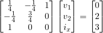
Thinking about the creation procedure, the [1, 1] entry is basically a sum between 0.25 and 0.5, which are caused by each of the two resistances. So, during the creation we will have duplicate entries for such cases! That's also a very important reason to why we are using COO in the first place, cause the other matrices don't store the duplicates and just keep the last occurrence. In other cases, this might be helpful, but for us it is not at all! After converting the COO matrix to CSR or CSC, the duplicates are summed up together, giving us exactly what we want...

So, let's fill in the triplets lists:

triplets = Triplet()

# add impact of R1
triplets.insert(0, 0, 0.25)
triplets.insert(0, 1, -0.25)
triplets.insert(1, 0, -0.25)
triplets.insert(1, 1, 0.25)

# add impact of R2
triplets.insert(1, 1, 0.5)

# add impact of V1
triplets.insert(0, 2, 1)
triplets.insert(2, 0, 1)

print(triplets, "\n")

This last print gives us:

We can clearly see that there are two entries for [1, 1], as we expected!

Last but not least let's also setup the actual matrix:

mtx = sparse.coo_matrix(
    (triplets.data, (triplets.rows, triplets.cols)), shape=(3, 3))

It will also be wise to delete the triplets using:

del triplets

Convert to more efficient Format (CSR/CSC)

Converting the COO format to CSR or CSC can be done veeeery easily using only one function call:

tocsr() - convert to CSR format
tocsc() - convert to CSC format

Doing each of these and printing out the format we have...

Can you guess, which one is CSR and which CSC? That's quite easy I think! We don't sort the entries, and so the "convertion" procedure left behind a very important mark. If you remember from last time, we loop through the matrix in either row-major order, which gives us CSR or column-major order, which gives us CSC. So, seeing that the first loops through each row and the second through each column first, we can understand that the first is CSR, whilst the second is CSC, even without knowing which function was used!

In code those two conversions are:

# convert to CSR
A = mtx.tocsr()

# convert to CSC
A = mtx.tocsc()

To print out the dense matrix we can use "todense()", which for both cases gives us:

Solving Linear System

We first have to define the numpy array of b:

b = np.array([0, 2, 3])

Solving the system is basically again just calling a function from a specific part of scipy.sparse that has to do with linear algebra solving. For now, we will use a direct solve approach that of course has to take in a sparse matrix (A) and dense matrix (b). More specifically this function can be imported from:

from scipy.sparse.linalg.dsolve import linsolve

Using this function to solve our system looks like this:

x = linsolve.spsolve(A, b)

Printing out the solution x we get:

which are the same results that we got without sparse matrices!

On GitHub I include the whole code for CSR and CSC...

Optimizing the Static Analysis Simulator

To optimize our current simulator, we basically only have to define the same Triplet class and insert the corresponding (row, column, value) pairs into the triplets lists. So, we will no longer have a numpy array for A, but will setup an instance of the Triplet class using:

triplets = Triplet()

While looping through the components and adding entries to the A-matrix, we will actually have to use the "insert()" function of Triplet. For example for voltage sources we now have:

elif component.comp_type == 'V':
    # affects the B and C matrices of A
    if high != 0:
        triplets.insert(high-1, g2Index, 1)
        triplets.insert(g2Index, high-1, 1)
    if low != 0:
        triplets.insert(low-1, g2Index, -1)
        triplets.insert(g2Index, low-1, -1)

    # affects b-matrix
    b[g2Index] = value

    # increase G2 counter
    g2Index = g2Index + 1

After the loop, we will use the triplet lists: data, rows and cols, to setup the actual sparse matrix in COO format, by then converting it to CSC format:

# setup sparse matrix A
    mtx = sparse.coo_matrix(
        (triplets.data, (triplets.rows, triplets.cols)), shape=(matrixSize, matrixSize))

    del triplets

    # convert to CSC
    A = mtx.tocsc()

The solving function of course has to be replaced with the new "sparse" one:

def solveSystem(A, b):
    x = linsolve.spsolve(A, b)
    return x

Running our Simulator for the simple example we get:

And so nothing really changed!

Running it for some of the other examples we would also see no different in the result values. So, what was this all for? As we also explained last time, Sparse matrices are of no use in such small Netlists, but will be essential for us when solving larger Netlists! Let's try to run the first Netlist from the following website:
http://tiger.cs.tsinghua.edu.cn/PGBench/index.html

Before we do so, we should first make sure to comment-out any printing...also let's point out that I forgot to take care of comments in the corresponding article, and that having zero g2-components and so g2Count = 0, would cause an indexing error. So, we have to tweak the following things:

...


# read netlist
    for line in file:
        # split line
        parts = line.split()
        # comment or option
        if(parts[0][0] == '*' or parts[0][0] == '.'):
            continue


...


# Group 2 component index
    if(g2Count > 0 ):
        g2Index = matrixSize - g2Count
    else:
        g2Index = 0

...

Running thupg1.spice we get:

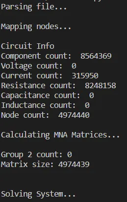
Not much information out of this, but still running it is impressive! It took up most of my computer's RAM, but before this optimization I couldn't run it at all, which tells something I think!

RESOURCES

References:

https://scipy-lectures.org/advanced/scipy_sparse/coo_matrix.html
https://scipy-lectures.org/advanced/scipy_sparse/csr_matrix.html
https://scipy-lectures.org/advanced/scipy_sparse/csc_matrix.html
https://scipy-lectures.org/advanced/scipy_sparse/solvers.html
https://docs.scipy.org/doc/scipy/reference/sparse.html

Mathematical Equations were made using quicklatex

Previous parts of the series

Introduction and Electromagnetism Background

Mesh and Nodal Analysis

Modified Nodal Analysis

Static Analysis

Sparse Matrix Optimization

Sparse Matrix Optimization (part 1)

Final words | Next up on the project

And this is actually it for today's post and I hope that you enjoyed it!

The articles from now on will be about Transient Analysis and "component extensions"...

So, see ya next time!

GitHub Account:

https://github.com/drifter1

Keep on drifting! ;)

Electronic Circuit Simulation - Sparse Matrix Optimization (part 2) [Python]