[Custom Thumbnail]

All the Code of the series can be found at the Github repository:
https://github.com/drifter1/circuitsim

Introduction

Hello it's a me again @drifter1! Today we continue with the Electronic Circuit Simulation series, a tutorial series where we will be implementing a full-on electronic circuit simulator (like SPICE) studying the whole concept and mainly physics behind it! In this article we will continue with the Modified Nodal Analysis Method, which is used to solve for voltages and currents, by creating the linear systems for Transient and Static Analysis and doing some examples on Static Analysis. In the next articles we will implement the complete simulator for Static Analysis, but following the suggestions of all the awesome utopian-io moderators, I will also make a Python implementation of today's examples, similar to the "by Inspection" Mesh and Nodal Analysis articles....

Requirements:

Physics and more specifically Electromagnetism Knowledge
Knowing how to solve Linear Systems using Linear Algebra
Some understanding of the Programming Language Python

Difficulty:

Talking about the series in general this series can be rated:

Intermediate to Advanced

Today's topic(s) can be rated:

Intermediate

Actual Tutorial Content

MNA System for Transient Analysis

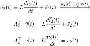
Using the various modifications and equations of the previous part (part 1) we can easily get the MNA System...

Let's first substitute the KVL Law that talks about components of Group 1 into the current equation of Group 1. By doing that the Current equation of Group 1 becomes:

Substituting this new equation of i₁(t) into KCL and doing some more calculations we get:

Let's now also substitute the KVL equation for Group 2 into the voltage equation of Group 2. That way we get the following mathematical equation:

Using the last two equations that we derived, we can write the following linear system, which is basically the MNA System of Transient Analysis:

In Matrix form this looks like this:

This is basically a linear system of (n-1) + m₂ equations...

MNA System for Static Analysis

In Static Analysis the voltage and current of the circuit are constant, meaning that v(t) and i₂(t) don't change over time. Thus, the MNA System for Static Analysis in matrix form is:

Thinking about the basic form of a linear system A·x = b, we can already understand which part of the matrix form corresponds to each part:

Let's now explain what exactly comes into each cell...

A-matrix

The A matrix is basically build up of 4 matrices: G, B, C and D. Each of them correspond to a specific part of the electronic circuit:

G is determined by the interconnections between the circuit elements and so basically showing the "effect" of conductance on the circuit
B is determined by the connection of the voltage sources and so showing the "effect" of voltage sources on the circuit
C is the transpose of B (when thinking about independent sources only)
D is all-zero when only independent sources are considered

So, we can rewrite the A-matrix as:

These matrices are filled following the rules:

A matrix

diagonal has positive sign, whilst rest is negative
each line and row corresponds to a specific node
the diagonal contains the total "self" conductance of each node
the non-diagonal entries contain the mutual conductance between the nodes

B matrix is an incidence matrix where each column corresponds to a specific voltage source and we put

1 when the node is connected to the + pole of the voltage source (basically meaning current leaves the node)
-1 when the node is connected to the - pole of the voltage source (basically meaning current enters the node)
0 when the node is not incident to the voltage source

C matrix - transpose of B (each row corresponds to a specific voltage source)
D matrix - all zero in Static Analysis

x-matrix

The x-matrix is giving us the solution: voltages and currents. More specifically it gives us:

the potential of each node of the circuit
the current that flows through all the group 2 components (basically voltage sources and Inductors for us)

b-matrix

The b-matrix contains the constant output of all independent sources of the circuit. The upper part corresponds to the current sources, whilst the rest are voltage sources. That way we basically never have zeros on the bottom, but only zeros in the upper part, as current sources don't really exist in every single node of the system. The sign that we put in front of the currents values goes by the following logic:

positive when the current is entering the node
negative when the current is leaving the node

Because of the negative sign in front of current sources inside of the b-matrix, the logic is exactly inverse to what we are used to! Let's also not forget that the voltage sources are always being put in positive, as the "direction" is already defined in the A-matrix.

Examples

To understand all this in practice, let's now get into two examples...

Example 1

Suppose that we have the following circuit:

As you can see we assigned the ground to the bottom node and named the nodes from left-to-right, by also giving a direction the current i_x that's leaving the voltage source. Therefore, the linear system for this circuit looks like this:

Let's explain the entries:

The "self" conductance of the nodes is G₁ = 1/4 and G₂ = 1/4+1/2 = 3/4, giving us those entries in the diagonal of G
The mutual conductance between the two only nodes that we have is:
G_{1, 2}=1/4. With a negative sign in front of it, this is the value that fills the final two cells of G
The B and C matrix of A, basically talk about the only voltage source that we have and how it connects to the nodes. As the current leaves node 1 we put '1' in the row of B (and column of C) that corresponds to node 1
The unknown quantities of the circuit are: v₁, v₂ and i_x, which fill the x-matrix in that exact order (potential first)
The current source doesn't connect to node 1 giving us a '0' in the first row of the b-matrix. Because it enters node 2, the second row of the b-matrix gets filled with the "positive" value '2' of the current source
The final row of the b-matrix is filled with the value of the voltage source which is '3'.

To solve for the unknown quantities we can write the following Python code:

import numpy as np

'''
Electronic Circuit is
+ ┌─R1 ┬────┐
  V1   R2   I1 ↑
- └────┼────┘
       ⏚

with following values:
'''
R1 = 4
R2 = 2
V1 = 3
I1 = 2

'''
Node 0: Connecting V1-R2-I1 (node at the bottom)
Node 1: Connecting V1-R1    (upper left node)
Node 2: Connecting R1-R2-I1 (upper right node)
'''

# Modified Nodal Analysis
a = np.array([[1/R1, -1/R1, 1],[-1/R1, 1/R1 + 1/R2, 0],[1, 0, 0]])
b = np.array([0, 2, 3])
print("A:\n", a, "\n")
print("b:\n", b, "\n")

# Solve System
x = np.linalg.solve(a,b)
print("x:\n", x)

Running this code we get the following results:

Example 2

Let's now suppose that we have the following circuit: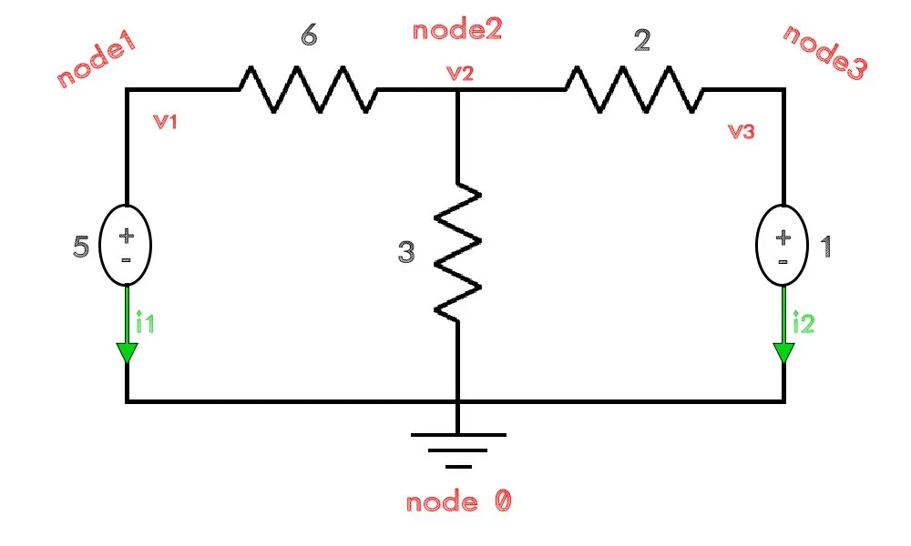

The linear system for this circuit is:

We can solve this problem by writing the following Python code:

import numpy as np

'''
Electronic Circuit is
+ ┌─R1 ┬─R3─┐ +
  V1   R2   V2 
- └────┼────┘ -
       ⏚

with following values:
'''
R1 = 6
R2 = 3
R3 = 2
V1 = 5
V2 = 1

'''
Node 0: Connecting V1-R2-V2 (node at the bottom)
Node 1: Connecting V1-R1    (upper left node)
Node 2: Connecting R1-R2-R3 (upper middle node)
Node 3: Connecting R3-V2    (upper right node)
'''

# Modified Nodal Analysis
a = np.array(
       [[1/R1, -1/R1, 0, 1, 0],
       [-1/R1, 1/R1 + 1/R2 + 1/R3, -1/R3, 0, 0],
       [0, -1/R3, 1/R3, 0, 1],
       [1, 0, 0, 0, 0],
       [0, 0, 1, 0, 0]   
       ])
b = np.array([0, 0, 0, 5, 1])
print("A:\n", a, "\n")
print("b:\n", b, "\n")

# Solve System
x = np.linalg.solve(a,b)
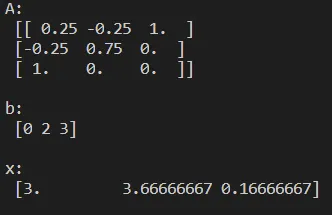
print("x:\n", x)

Running it we get the following results:

All this is still "manual", but already giving us the idea of what we will be doing next time to create a full electronic circuit simulator for Static Analysis! First up we will of course have to find a way to store the information of a net-list efficiently, so that the components can then be "mapped" into nodes and so rows/columns of the MNA matrices. After we have successfully created the MNA system, solving it is very easy...just a call of linalg.solve().

RESOURCES

References:

http://qucs.sourceforge.net/tech/node14.html

Mathematical Equations were made using quicklatex

Previous parts of the series

Introduction and Electromagnetism Background

Mesh and Nodal Analysis

Modified Nodal Analysis

Final words | Next up on the project

And this is actually it for today's post and I hope that you enjoyed it!

Next time we will start with the Implementation of the Electronic Circuit Simulator for Static Analysis, where you will see why the theoretical talk was worth it! So, see ya next time!

GitHub Account:

https://github.com/drifter1

Keep on drifting! ;)

Electronic Circuit Simulation - Modified Nodal Analysis (part 2) [Python]