[Custom Thumbnail]
All the Code of the series can be found at the Github repository:
https://github.com/drifter1/circuitsim
Introduction
Hello it's a me again @drifter1! Today we continue with the Electric Circuit Simulation series, a tutorial series where we will be implementing a full-on electronic circuit simulator (like SPICE) studying the whole concept and mainly physics behind it! In this article we will start getting into the so called Modified Nodal Analysis Method, which is used to solve for voltages and currents. Explaining this method and implementing it in Python will take some explaining and so this topic will be split into parts...Requirements:
- Physics and more specifically Electromagnetism Knowledge
- Knowing how to solve Linear Systems using Linear Algebra
- Some understanding of the Programming Language Python
Difficulty:
Talking about the series in general this series can be rated:- Intermediate to Advanced
- Intermediate
Actual Tutorial Content
Circuit Component Groups
Thinking about the various components of electronic circuits (resistors, capacitors, inductors, voltage and current sources), we easily come to the conclusion that the mathematical equation that describes them can either be solved in respect to current, voltage or both. Remembering that Nodal Analysis is based on KCL and so calculating the voltages, we only have problems with components that cannot be solved in respect to current, but only voltage. So, which "basic" components can and which cannot we written in respect to current?Group 1 (can be written)
Current source
The simplest one is the independent current source, which constantly outputs current (either DC or TC). The equation that describes a current source is:
where:
- si is the current of a current source over time
- ai is the constant DC part of a current source
- fi(t) is the TC part as a function over time
So, for Static Analysis a current source will just output a constant value...
Resistor
Another quite simple case is the resistor. Thinking about Ohm's Law, the equation of a resistor can easily be written in respect to current, voltage or resistance. Therefore, the equation that describes the current of a resistor is:
As you can see we can easily replace Resistance with Conductance...
Capacitor
In part 2 of the Electromagnetism Background (3rd article) using the general equation of a capacitor and the definition of current as the charge over time, we ended up with the following equation that describes the current of a capacitor over time:
Don't get confused by the use of the letter 'u'. Last time we explicitly explained that voltage is symbolized by 'u', whilst the potential of a node in respect to a reference node is written as 'v'.
Combined Equation
We can easily combine current sources, resistors and capacitors, to write the following equation for any circuit component 'k' of Group 1:
Group 2 (cannot be written)
Voltage source
The component that made analysis more difficult using Nodal Analysis was the voltage source. Quite similar to the current source, the equation that describes a voltage source is:where:
- sv is the voltage of a voltage source over time
- av is the constant DC part of a voltage source
- fv(t) is the TC part as a function over time
For Static Analysis a voltage source will just be the part av...
Inductor
Even though we can basically solve for the current of an Inductor using the Integral:
we tend to use the equation of Electromagnetic Induction that is giving us the induced voltage of an inductor:

Combined Equation
Similar to Group 1, we can also combine voltage sources and inductors to write the following equation for any circuit component 'k' of Group 2:
Matrix and Vector Modifications
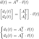
Dividing the circuit components into these groups, we clearly have to change the matrices and vectors of our circuit analysis methods now. More specifically, we will split the (reduced) incidence matrix A into two matrices A1 and A2 (one for each group), by also splitting the vectors i(t) and u(t) into two vectors each. Vector v(t) of node potentials doesn't have to be split. Supposing that the total number of components is m, the total number of components in group 1 is m1 and the total number of components in group 2 is m2 (m1 + m2 = m), we can write the incidence matrix Aas:
Similarly, the vectors become:


KCL and KVL Laws
Using this "splitting" of matrices and vectors we clearly have to rewrite KCL and KVL...Group-KCL

Group-KVL
Group Equations
Let's revisit the Group Equations again, now that we know which exact vectors come into the equations. Putting vectors we will basically create systems of equations...Group 1 Equations
Using the vectors i1(t) and u1(t) the combined equation of Group 1 becomes:
Group 2 Equations
Using the vectors i2(t) and u2(t) the combined equation of Group 2 becomes:
RESOURCES
References:
- http://qucs.sourceforge.net/tech/node14.html
Mathematical Equations were made using quicklatex
Previous parts of the series
- Introduction
- Electromagnetism Background (part 1)
- Electromagnetism Background (part 2)
- Mesh Analysis
- Nodal Analysis
- Modified Mesh Analysis by Inspection
- Modified Nodal Analysis by Inspection
- Incidence Matrix and Modified Kirchhoff Laws
Final words | Next up on the project
And this is actually it for today's post and I hope that you enjoyed it!Next time we will cover the MNA Systems of Transient and Static Analysis, by also doing detailed examples on Static Analysis...
So, see ya next time!
GitHub Account:
https://github.com/drifter1
Keep on drifting! ;)