[Custom Thumbnail]

All the Code of the series can be found at the Github repository:
https://github.com/drifter1/circuitsim

Introduction

Hello it's a me again @drifter1! Today we continue with the Electric Circuit Simulation series, a tutorial series where we will be implementing a full-on electronic circuit simulator (like SPICE) studying the whole concept and mainly physics behind it! In this article we will modify the Mesh Analysis Method by Inspection, to create the linear system more easily.

Requirements:

Physics and more specifically Electromagnetism Knowledge
Knowing how to solve Linear Systems using Linear Algebra
Some understanding of the Programming Language Python

Difficulty:

Talking about the series in general this series can be rated:

Intermediate to Advanced

Today's topic(s) can be rated:

Intermediate

Actual Tutorial Content

Mesh Analysis Method (Recap)

To recap really quick, Mesh (Current) Analysis is based on Kirchhoff's Voltage Law (KVL) and so calculating the current in the various meshes of an electronic circuit (mesh currents). The steps of this method are:

Identify the meshes of the circuit
Assign mesh currents to each mesh
Write the KVL equations
Solve the linear system
Solve for other element currents and voltages

Modifying by Inspection

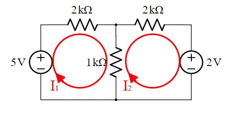
In the 4th article of the series we explained the method very in-depth, solving an example using this method "by hand" and using "manual" Python Code. By the end of the article, during the Python Implementation we found out that the A-matrix contains only Resistances, whilst the b-matrix contains only Voltages, which already gave us an idea to what is coming today! But, we never really explained what exactly comes into each "cell" or coefficient of the linear system.

The example circuit that we solved back then was:

To solve the circuit we basically created the following linear system:

By inspecting the resulting Linear System of this example we see that:

The A-matrix contains only Resistances and:

the diagonal has a positive sign, whilst the rest is negative
each line and row is about a specific mesh
the diagonal contains the total "self" resistance of each mesh
the non-diagonal entries contain the mutual resistance between the meshes

The b-matrix contains only Voltages and:

each row talks about a specific mesh
we put a positive sign if the current flows - → +
we put a negative sign if the current flows + → -

So, to generalize for any circuit, let's define some "rules"...

Resistance Matrix

The general form of the Resistance matrix for n-meshes is:

Each entry gets filled based on the following rules:

If the entry is referring to the same mesh (E.g. R_a,a), we fill it with the total "self" resistance of the corresponding mesh
If the entry is referring to different meshes (E.g. R_a,b) we fill it with the "negative" mutual resistance of the two meshes

Voltage Matrix

The general form of the Voltage matrix for n-meshes is:

Each entry gets filled based on the following rules:

The entry is equal to the sum of all voltage sources that occur in the corresponding mesh
The sign of each voltage in the sum depends on "how" the current flows through the voltage source:

positive sign if the current flows - → +
negative sign if the current flows + → -

Linear System

So, the general form of the whole linear system is:

Manual Python Implementation

Let's now solve another example that is more complicated, by just filling in the cells of the linear system's matrices using this new modified method!

Suppose that we have the following circuit:

[Image 1]
with the following resistance and voltage values:

The linear system for this circuit looks like that:

The Python code that solves this problem looks like this:

import numpy as np

'''
Electronic Circuit is
┌ R1 ┬ R2 ┬ R3 ┐
│    R4    R5   R6
└ V1 ┴────┴ V2 ┘
 -  +      -  +
with following values:
'''
R1 = 5
R2 = 10
R3 = 3
R4 = 7
R5 = 4
R6 = 1
V1 = 1
V2 = 3

'''
Mesh 1: V1-R1-R4 Loop
Mesh 2: R4-R2-R5 Loop
Mesh 3: V2-R5-R3-R6 Loop

Mesh Currents (all clockwise)
I1 for Mesh 1
I2 for Mesh 2
I3 for Mesh 3
'''

# Modified Mesh Analysis By Inspection
a = np.array([[R1 + R4, -R4, 0],[-R4, R2 + R4 + R5, -R5], [0, -R5, R3 + R5 + R6]])
b = np.array([-V1, 0 , -V2])
print("A:\n", a, "\n")
print("b:\n", b, "\n")

# Solve System
x = np.linalg.solve(a,b)
print("x:\n", x)

Running this code we get the following:

So, the mesh currents are:

RESOURCES

References:

http://www.eeeguide.com/mesh-analysis-equation/

Images:

https://electronics.stackexchange.com/questions/158613/why-does-the-mesh-currents-method-work

Mathematical Equations were made using quicklatex

Previous parts of the series

Final words | Next up on the project

And this is actually it for today's post! I hope that I was able to explain everything as much as needed!

Next up on this series we will modify the other method that we covered (Nodal Analysis) by Inspection to create the Linear System somewhat automatically...

So, see ya next time!

GitHub Account:

https://github.com/drifter1

Keep on drifting! ;)

Electronic Circuit Simulation - Modified Mesh Analysis by Inspection [Python]