
Hello its me again drifter1. Today we continue with Mathematical Analysis getting into Taylor and Maclaurin Power Series. You should check out my previous post about Power Series first here. So, without further do, let's get straight into it!
Taylor and Maclaurin Series Theory:
We already said that a function can be represented as a Power Series like that:

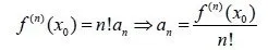
Now we have to find the coeffiecients ai.
For a0 we simply have f(x0) = a0
For the rest we find the derivatives of f(x)...

That way we see that the function f(x) can be represented in another way like that:

So, the ai parts now are gone and we ended up with another form.
Taylor polynomial:
The same representation of f as before, but for a specific n value is the so called Taylor polynomial with n-degree of the function f.
This looks like that:

Taylor series:
The power series with center x0 that represents f(x) is called the taylor series of f and looks like this:

Maclaurin series:
By setting the center x0 equal to 0 we end up with a special case of the Taylor series that is called a Maclaurin series (with center 0) and looks like this:

Function value approximation:
From all that you can see that we can approximately calculate the value of any function by using n terms of this series. Sometimes we don't even have to do it on n-parts, but can directly find the limit for an specific x value.
There are some ways to calculate the error using the Lagrange or Cauchy Remainder that I will not cover, but you can check them out if you want to.
So, lets get into some Examples now, but only for Maclaurin that is simpler :P
Maclaurin Function Representation Examples:
f(x) = e^x :
- Find the Macluarin Series for f(x)
- Find the 5-degree and 8-degree polynomials.
- Calculate the values of p5(1) and p8(1), how big is the offset?
1.
e^x is a function whose derivative equals the same function for any natural n-derivative.
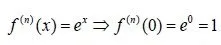
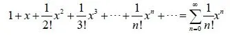
So, the Maclaurin Series looks like this:
2.
For n = 5 we end up with:

For n = 8 we end up with:

3.
For x =1 we end up with:
p5(1) = 2.71666...
p8(1)= 2.71827876...
The actual value of e = 2.71828128284590...
We see that with a degree of 5 we end up with the first 2 decimal digits right and with a degree of 8 with 4 right! So, by using this series that contains factorial we end up with a close approximation with just a little terms.
g(x) = sin(x) and h(x) = cos(x) :
Find the Maclaurin Representation of g (1.) and h (2.)
1.
We know that the sin(x) derivative can get one of 4 values and depends on the value of the degree.
For the first 4 derivative we end up with:
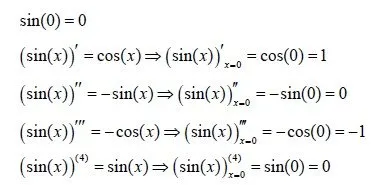
Using mathematical substitution we can find out that the following applies to n:
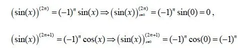
For even value the value of the coeffiecients is 0 and for odd it is (-1)^n.
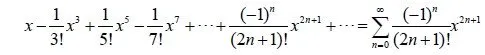
So, using only the odd terms we end up with the Maclaurin Representation that looks like this:
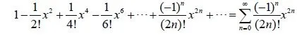
2.
In the same way as before we will find the first 4 terms and the use mathematical substituion that I again will leave out for simplicity reasons.
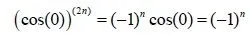
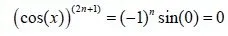
So, this time the odd terms are 0 and we use only the even terms and end up with:
Here you can see the Maclaurin Representations of common functions. I think that these 3 examples are more then enough for you to understand the basics and the usage of these series. We will get back to this representation later on when we get into Arithmetic Methods that let us calculate the value of a function, derivative, integral or even differential equations in a repetitive way.
And this is actually it for today and I hope that you enjoyed it!
Next time we will get into the final part of Series (and Mathematical Analysis for now) and talk about the Fourier Series that is pretty useful too.
Bye!