Hello it's a am again. Today we continue with Linear Algebra getting into Linear Functions Matrixes and also some special cases. Last time we covered the basics of Linear Functions. So, without further do let's get started!
Linear Function Matrix:
Suppose two vector spaces V and W with Bv = {v1, v2, ..., vn} being a basis of V and Bw = {w1, w2, ..., wm} a basis of W. As we said last time, we can construct a linear function f: V -> W, determining that f(vi) (1<=i<=n) are the images of the basis vectors of Bv.
Then the image of every vector x = k1*v1 + k2*v2 + ... + kn*vn of V, where ki are real is defined as:
f(x) = k1*f(v1) + k2*f(v2) + ... + kn*f(vn)
The images of f(vi) (1<=i<=n) as vector of W can be written as linear combinations of the basis vectors of Bw.
Let's say those are:
f(v1) = a11*w1 + a21*w2 + ... + am1*wm
f(v2) = a12*w2 +a22*w2 + ... + am2*wm
..................................................................
f(vn) = a1n*w1 + a2n*w2 + ... + amn*wm
where aij is a real number and 1<=i<=m and 1<=j<=n
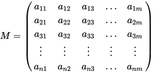
That way we can construct a matrix using the coefficients of aij that is called the linear function matrix or linear morphism matrix.
We get these coefficients from the bases Bv and Bw of the vector spaces V and W.
So, we can define this function also using:
f(v) = A*v, for every v in V
Example:
Suppose a linear morphism f: R^3 -> R^3, where f(x, y, z) = (x + 2y + z, x + 5y, z).
We will use the standard basis {e1, e2, e3} of R^3, where e1 = (1, 0, 0), e2 = (0, 1, 0) and e3 = (0, 0, 1).
That way we have:
f(e1) = (1, 1, 0) = 1*e1 + 1*e2 + 0*e3
f(e2) = (2, 5, 0) = 2*e1 + 5*e2 + 0*e3
f(e3) = (1, 0, 1) = 1*e1 + 0*e2 + 1*e3
So, the function matrix is:
1 2 1
1 5 0
0 0 1
Transition Matrix:
The square matrix that we get from the indicator function Iv: V -> V from the bases B1 = {v1, v2, ..., vn} and B2 = {u1, u2, ...un} is called a transition matrix from basis B1 to B2. We write it as PB1->B2.
That way the transition matrix has the coordinates of the vectors of basis B1 when in basis B2.
This means that:
[v1 v2 ... vn] = [u1 u2 ... un]*PB1->B2
In the same way we can get:
[u1 u2 ... un] = [v1 v2 ... vn]*PB2->B1
Invertibility:
For any two bases B1, B2 of V we know that PB2->B1*PB1->B2 = In (indicator matrix)
So, PB1->B2 = PB2->B1^-1 (inverse) and so the transition matrix is invertible.
We can also say tha same for the other way around:
PB2->B1 = PB1->2^-1 (inverse)
Isomorphism Theorem:
Suppose V, W are two vectors spaces and Bv = {v1, v2, ..., vn} is a basis of V and Bw = {w1, w2, ..., wm} a basis of W. If f is a function in the homomorphism Hom(V, W) and A is a the morphism matrix that we get from f when going from Bv to Bw then:
Hom(V, W) -> M mxn, transitioning using homomorphism h having f->A using the same h.
The function Hom(V, W) -> M mxn is a isomorphism.
When V and W are vector spaces and dimV = n, dimW = m then dimHom(V, W) = m*n.
When A is the mxn function matrix of f: V->W on the bases Bv and Bw then:
- N(A) = Kerf
- dimImf = rank(A)
When the the function f is also a homomorphism (f: V->V) we know that the matrix A^-1 (inverse matrix of A) is correspnding to the function f^-1 that is the inverse function of f.
Equality and Similarity:
Two mxn matrixes A, B are equivalent when there are two invertible matrixes P in M^m and S in M^n so that:
B = P^-1*A*S
Two square matrixes A, B are similar when there is a invertible matrix P in M^n so that:
B = P^-1*A*P
When f: V->V is a homomorphism of V and A is the function matrix with basis B = {v1, v2, ..., vn} and B is a function matrix of basis B' = {v1', v2', ..., vn'} then A and B are similar.
Special Cases:
A function that is of the form f: R^2 -> R^2, where f(x, y) = (ax, ay) and a in R is called a expansion when a>=1 and a compression when 0<a<1.
The function matrix can be represented as:
a 0
0 b
When a = 1: we move in the y'y axis
When b = 1: we move in the x'x axis
We can also define a rotation function where (x, y) ->(xcosφ + ysinφ, -xsinφ + ycosφ)
That way the function matrix looks like this:
cosφ -sinφ
sinφ cosφ
We can also define the projection Pr of a line with angle θ and the matrix looks like this:
cos^2θ cosθ*sinθ
cosθ*sinθ sin^θ
And this is actually it for today and I hope you enjoyed it!
Next time in Linear Algebra we will get into eigenvalues and eigenvectors.
Bye!