Hello it's a me Drifter Programming! Today is the last "Theory" post of Logic Design and we will talk about Binary Decision Diagrams. After that I have one more Multisim Implementation post and then we will get into VHDL Circuit Coding (maybe even Verilog sometime later on). So, without further do let's get started!
Introduction:
BDD's are another way of representing a Boolean Function. It is a datastructure similar to a Graph that represents the relations between the variables. This Graph contains decision and terminal Nodes. The decision Nodes are labeled with the names of the Boolean Variables. The terminal Nodes can be either 0 or 1 and represent the Output of our function. The Edges that connect those Nodes represent assigments of 0 or 1 to those Variables.
We mostly reduce/simplify the BDD Graphs even more merging isomophic subgraphs into one. This type of BDD Graph is called a Reduced Ordered Binary Decision Diagram (ROBDD). We use ROBDD Graphs instead cause this Graphs are unique for a particular function and variable Order! A function with N variables can have 2^N different Input combinations. The functions that we can have are 2^2^N, cause the Output for each Input combination can be either 0 or 1.
So, to recap really quick. BDD's represent Boolean Functions and are Graphs with Nodes that represent Boolean variables (decision Nodes) and Outputs (terminal Nodes), and Edges that represent assignments. We mostly use a reduced form called ROBDD, cause this Graph is unique for each particular function.
Let's first start talking about Binary Decision Trees that are simple to understand, then get into BDD's and lastly after that we can get into ROBDD's as well.
Binary Decision Trees:
Binary Decision Trees are pretty easy to make, but can get really really big. With N variables we will have 2^N-1 Decision Nodes and 2^N Edges! A nice property (canonicity) they have is that when testing out variables in a fixed order the binary decision tree is unique! To compare 2 functions we will need to have the 2 BDT's ordered in the same way.
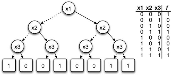
Look at the BDT for a XOR Function (x1⊕x2) for example:
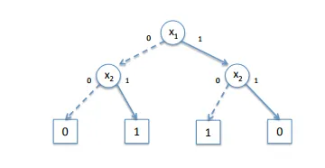
You can see that we started out with x1 and created 2 subtrees: one for x1 = 0 and one for x1 = 1. Then we had to check x2 in the same way, finishing off with the output in Terminal Nodes of 0 or 1.
I hope that you can see that if we continue on this process we will have 1, 2, 4, 8,..., 2^N Nodes in each new Level of our Tree that makes our Tree gigantic and complicated in no time.
So, what do we do then? Well we don't use BDTrees, but BDDiagrams that are Graphs and let us connect Nodes with more than 2 other Nodes and also let us remove Decision Nodes that are not needed in specific Cases where this variable doesn't change the Output when it already is 1 by another "minterm" of our function.
Binary Decision Diagrams:
BDD's are better than BDT's, cause they have 2 improvements, but they have no canonicity. One of the improvements is that we can leave out variables in some branches (redundancies). Think of an Multi-AND Gate, where one of the Variables is already 0. There is no need to test any of the other Variables, cause the Output will be 0 either way!
So, an BDD for an AND Function (x1ANDx2) looks like this:
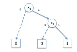
You can see that we left out x2 when x1 = 0. That way we made our BDD contain less Nodes, cause we deleted 1 Decision Nodes that would give us 2 Terminal Nodes, from which we have 1 now! So, instead of 7 we have 5 Nodes in total.
Secondly, we can share identical subtrees. That means that we can connect an assignment Edge to an already existing Node instead of creating a new Node everytime, when the Nodes contained inside of this subtree are the same (identical). Think of an function that gives us 1 when we have odd parity (odd number of 1's in input) and 0 when we have even parity( even number of 1's in input). Some parts can be shared and that way instead of 15 Decision Nodes and 2(or 16) Derminal Nodes we can have 7 Decision Nodes and 2 Terminal Nodes.
The BDD for this odd parity checking function looks like this:
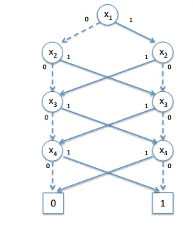
You can see that we cross-combined the Decision Nodes so that we minimize the BDD size. We also included only 2 Terminal Nodes, cause making the BDD contain Subtrees there is no need for more then 2.
So, to sum up. In the worst case our BDD will be actually a BDT. But, in the most practically occuring cases it will be much smaller. One thing that makes a BDD always smaller than a BDT is that we can simply use 2 Terminal Nodes that represent the 2 different Outputs our function can have.
Reduced Ordered Binary Decision Diagrams:
A ROBDD is a BDD that is based on a fixed ordering of variables and is also reduced. Reduced means that Irredundancy and Uniqueness apply. The first means that the low and high successors of every node are distinct. The second means that there are no two distinct nodes testing the same variable with the same successors. That way ROBDD's recover the canonicity property that makes our Graph be unique for each boolean function and fixed variable ordering. That way we can compare to functions by comparing their ROBDD's.
One way of constructing such a ROBDD Graph is by creating a BDD and then eliminating redundancies and identifying identical subtrees. But, this takes too much time when having a big BDD Graph and so we must find another way. We can also create a ROBDD by following the structure of our boolean expression that defines the function. We will create a ROBDD for each part of our function decomposing it even into the variable level. Then we will combine those parts together into a new ROBDD by following the boolean operation with which this two ROBDD Elements were connected inside of the function continuously, until we have our final ROBDD Graph.
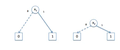
Let's get into an Example for the function F(x1, x2) = x1 ⊕ x2 = (x1 + x2) (x1' + x2') following the order x1 < x2. We will first create a BDD for each Variable. Then we will create a ROBDD for each of the OR Operations. Lastly we will combine those 2 OR Operations with the final AND Operation.
x1 and x2 look like this (the opposite is x1' and x2'):
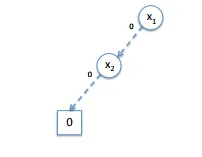
To combine (x1 + x2) we fill do it in 2 passes. First with the low (left) successor and then with the high (right) successor. Following the low successor we will find the Output 0 part and following the high successor the Output 1 part of our ROBDD Diagram.
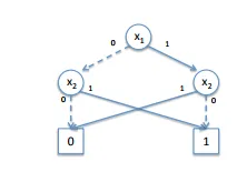
If we then follow the Output 1 part and remove redundancies we finally end up with (x1 + x2) looking like this:

(x1' + x2') is exactly the opposite and looks like this:

So, combining those 2 again we end up with the following ROBDD for our function (you can check it out by ourself):
I got help from this Lecture and you can check it out for more information in some regions if you wish!
And this is actually it! Hope you enjoyed this post!
I don't wanted to make it too complicated, but just explain what BDD's are all about. Off course I could have done it much bigger, but this was just a topic that I wanted to point out for those that may be interested in. Next time we will implement an Advanced Sequential Circuit using JK Flip Flops in Multisim and this will also be the last post in Logic Design before getting into VHDL Coding!
Until next time...Bye!