[Image1]
Introduction
Hey it's a me again @drifter1!
Today we continue with my mathematics series about Signals and Systems to get into Exercises on Linear Feedback Systems.
So, without further ado, let's dive straight into it!
Linear Feedback System Response Examples (Based on 25.4 from Ref1)
Consider simple feedback systems in continuous- and discrete-time respectively, as shown in the figure below.
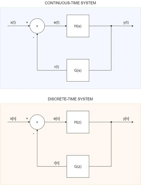
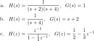
Let's determine the closed loop system impulse response, v(t), for the continuous-time system, and system function, V(z), for the discrete-time system, in each of the following cases:
Solution
For both systems, the closed loop system function can be defined as:

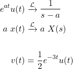
a.
For the first case, the system function is:

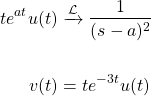
Thus, from the Laplace Transform tables:
b.
In the second case, we have:

Which, using the Laplace Transform tables and linearity property, yields the impulse response:
c.
The third case and final case is for the discrete-time system. The closed loop system function is as follows:
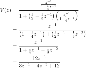
In the Z-Transform the calculations tend to become quite tedious,
and coming up with examples that simplify is also quite difficult.
So, let's just leave it there...
Linear Feedback System Stability Example (Based on 25.6 from Ref1)
Let's consider the causal discrete-time shown below.

- a. Proof that the system is not stable
- b. Suppose that there's feedback with one unit of delay, which means that the input is now given by:

where xe[n] is now the input to the overall system.
Determine the range of values of K (if such values exist) for which the system is stable.
Solution
a.
In order to prove that the system is not stable, we have to proof that at least one pole is at |z| > 1. So, let's first find the system function that describes the system.
As a difference equation the system can be written as:

Taking the Z Transform of the equation yields:

The solutions of the denominator are the poles of the system. So, the poles of the system are located at:

Since |z1| = 2 > 1, the system is unstable.
b.
Introducing feedback of one unit of delay, the difference equation changes into:

Taking the Z Transform yields the system function:

The poles are now located at:

For z = 1 we can find the range of K

The root term inside the square root is always positive, thus the roots are purely real. So, squaring both sides of the equation gives us the solution(s):

Heading back, z is now:

So, the |z| < 1 condition is not satisfied. Thus, the system is not stable.
You could keep going with two, three etc. units of delays as homework, until the system becomes stable!
RESOURCES:
References
Images

Mathematical equations used in this article were made using quicklatex.
Block diagrams and other visualizations were made using draw.io
Previous articles of the series
Basics
- Introduction → Signals, Systems
- Signal Basics → Signal Categorization, Basic Signal Types
- Signal Operations with Examples → Amplitude and Time Operations, Examples
- System Classification with Examples → System Classifications and Properties, Examples
- Sinusoidal and Complex Exponential Signals → Sinusoidal and Exponential Signals in Continuous and Discrete Time
LTI Systems and Convolution
- LTI System Response and Convolution → Linear System Interconnection (Cascade, Parallel, Feedback), Delayed Impulses, Convolution Sum and Integral
- LTI Convolution Properties → Commutative, Associative and Distributive Properties of LTI Convolution
- System Representation in Discrete-Time using Difference Equations → Linear Constant-Coefficient Difference Equations, Block Diagram Representation (Direct Form I and II)
- System Representation in Continuous-Time using Differential Equations → Linear Constant-Coefficient Differential Equations, Block Diagram Representation (Direct Form I and II)
- Exercises on LTI System Properties → Superposition, Impulse Response and System Classification Examples
- Exercise on Convolution → Discrete-Time Convolution Example with the help of visualizations
- Exercises on System Representation using Difference Equations → Simple Block Diagram to LCCDE Example, Direct Form I, II and LCCDE Example
- Exercises on System Representation using Differential Equations → Equation to Block Diagram Example, Direct Form I to Equation Example
Fourier Series and Transform
- Continuous-Time Periodic Signals & Fourier Series → Input Decomposition, Fourier Series, Analysis and Synthesis
- Continuous-Time Aperiodic Signals & Fourier Transform → Aperiodic Signals, Envelope Representation, Fourier and Inverse Fourier Transforms, Fourier Transform for Periodic Signals
- Continuous-Time Fourier Transform Properties → Linearity, Time-Shifting (Translation), Conjugate Symmetry, Time and Frequency Scaling, Duality, Differentiation and Integration, Parseval's Relation, Convolution and Multiplication Properties
- Discrete-Time Fourier Series & Transform → Getting into Discrete-Time, Fourier Series and Transform, Synthesis and Analysis Equations
- Discrete-Time Fourier Transform Properties → Differences with Continuous-Time, Periodicity, Linearity, Time and Frequency Shifting, Conjugate Symmetry, Differencing and Accumulation, Time Reversal and Expansion, Differentation in Frequency, Convolution and Multiplication, Dualities
- Exercises on Continuous-Time Fourier Series → Fourier Series Coefficients Calculation from Signal Equation, Signal Graph
- Exercises on Continuous-Time Fourier Transform → Fourier Transform from Signal Graph and Equation, Output of LTI System
- Exercises on Discrete-Time Fourier Series and Transform → Fourier Series Coefficient, Fourier Transform Calculation and LTI System Output
Filtering, Sampling, Modulation, Interpolation
- Filtering → Convolution Property, Ideal Filters, Series R-C Circuit and Moving Average Filter Approximations
- Continuous-Time Modulation → Getting into Modulation, AM and FM, Demodulation
- Discrete-Time Modulation → Applications, Carriers, Modulation/Demodulation, Time-Division Multiplexing
- Sampling → Sampling Theorem, Sampling, Reconstruction and Aliasing
- Interpolation → Reconstruction Procedure, Interpolation (Band-limited, Zero-order hold, First-order hold)
- Processing Continuous-Time Signals as Discrete-Time Signals → C/D and D/C Conversion, Discrete-Time Processing
- Discrete-Time Sampling → Discrete-Time (or Frequency Domain) Sampling, Downsampling / Decimation, Upsampling
- Exercises on Filtering → Filter Properties, Type and Output
- Exercises on Modulation → CT and DT Modulation Examples
- Exercises on Sampling and Interpolation → Graphical/Visual Sampling and Interpolation Examples
Laplace and Z Transforms
- Laplace Transform → Laplace Transform, Region of Convergence (ROC)
- Laplace Transform Properties → Linearity, Time- and Frequency-Shifting, Time-Scaling, Complex Conjugation, Multiplication and Convolution, Differentation in Time- and Frequency-Domain, Integration in Time-Domain, Initial and Final Value Theorems
- LTI System Analysis using Laplace Transform → System Properties (Causality, Stability) and ROC, LCCDE Representation and Laplace Transform, First-Order and Second-Order System Analysis
- Exercises on the Laplace Transform → Laplace Transform and ROC Examples, LTI System Analysis Example
- Z Transform → Z Transform, Region of Convergence (ROC), Inverse Z Transform
- Z Transform Properties → Linearity, Time-Shifting, Time-Scaling, Time-Reversal, z-Domain Scaling, Conjugation, Convolution, Differentation in the z-Domain, Initial and Final value Theorems
- LTI System Analysis using Z Transform → System Properties (Causality, Stability), LCCDE Representation and Z Transform
- Exercises on the Z Transform → Z Transform and ROC Examples, ROC from Conditions, LTI System Analysis Example
- Continuous-Time to Discrete-Time Design Mapping → Discrete-Time System Design Techniques (Mapping from Derivatives to Differences, Mapping using Impulse Invariance), First- and Second-Order Systems and Z-Transform
- Butterworth Filters → Butterworth Filter Parameters, Equation and Pole-Zero Plot, Mapping using Impulse-Invariance and Bilinear Transformation
- Linear Feedback Systems → System Feedback, Linear Feedback System Analysis
Final words | Next up
This might actually be the end of the series, I'm not sure if there's much more to cover...
Also, this kind of posting has become quite boring and repetitive, so I'm looking for ways to spice things up. Maybe more coding, maybe more actual examples and exercises in these types of subjects (which are more on the theoretical side of things)...we shall see! But, you can be certain that the diversity of content will be enhanced thoroughly, because of the introduction of videos and maybe even streaming.
No more Mr. Text-guy!

Keep on drifting!