[Image1]
Introduction
Hey it's a me again @drifter1!
Today we continue with my mathematics series about Signals and Systems in order to cover Continuous-Time Modulation.
So, without further ado, let's dive straight into it!
Modulation Property
Let's first recall what modulation means in the context of Signals and Systems. Modulation is one of the various useful properties of the Fourier Transform, and is basically the FT of the multiplication of two signals. As we know, the product/multiplication of two signals turns into a convolution of their individual Foruier Transforms.
Consider x(t) to be the continuous-time signal to be "modulated".
The signal c(t) which is used to modulate x(t) is known as the carrier signal.
Various types of carriers can be used, which we will get into in a bit.
As a result, the modulation property can be written as:

Getting into Modulation
Modulation is a very important concept used in communication systems, and also the basis for converting between continuous-time and discrete-time signals. To put things simply, think of the information being embedded into the carrier signal by tweaking/modulating some parameter of it.
The two basic modulations are amplitude and frequency modulation. In amplitude modulation, the information to be transmitted modulates the amplitude of the carrier, whilst the carrier signal that transmits it is a sinusoidal signal of specific frequency. On the other hand, in frequency modulation, the information modulates the frequency of the carrier, transmitting the information in the amplitude of the carrier signal.
So, remember the following:
- Amplitude Modulation (AM) = Transmission in the Frequency of the Carrier Signal
- Frequency Modulation (FM) = Transmission in the Amplitude of the Carrier Signal
Amplitude Modulation
Let's start of with amplitude modulation.
Graphically, AM looks as follows:

[Image 2]
AM is defined by the simple modulation/property that we covered before, and so the outcome is as follows:

The carrier signal can be a:
- pulse signal
- sinusoidal signal

- complex exponential signal


Frequency Modulation
Next up is FM, which graphically does the following:
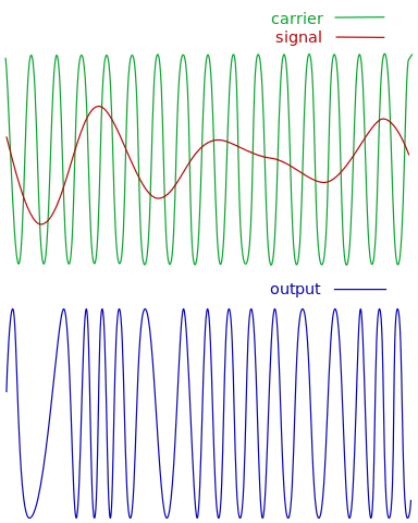
[Image 3]
In FM, the frequency of the carrier is modulated, which in turns means that the the input signal modulates the phase of the carrier signal in some manner.
Using a sinusoidal carrier, its easy to define FM as:

Tweaking the parameter k allows us to widen/narrow the bandwidth of the transmission.
If we applied x(t) directly, the outcome would be Phase Modulation (PM):

Demodulation
In addition to modulation there is also the concept of demodulation. Using a complex exponential carrier the original signal can be recovered very easily, by modulating a second time using the complex conjugate signal.

Contrarily, the recovery of the signal using a sinusoidal carrier is a two step procedure. Demodulation consists of modulating again with a sinusodial carrier, followed by low-pass filtering that "extracts" the original signal.
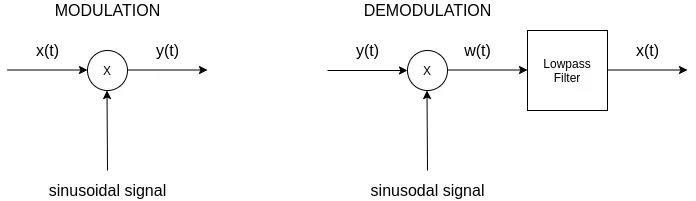
Because synchronization is quite difficult to achieve, demodulation is easier to implement asynchronously. But, such a less expensive demodulator suffers of inefficiency in power transmission.
RESOURCES:
References
Images


Mathematical equations used in this article were made using quicklatex.
Block diagrams and other visualizations were made using draw.io and GeoGebra
Previous articles of the series
Basics
- Introduction → Signals, Systems
- Signal Basics → Signal Categorization, Basic Signal Types
- Signal Operations with Examples → Amplitude and Time Operations, Examples
- System Classification with Examples → System Classifications and Properties, Examples
- Sinusoidal and Complex Exponential Signals → Sinusoidal and Exponential Signals in Continuous and Discrete Time
LTI Systems and Convolution
- LTI System Response and Convolution → Linear System Interconnection (Cascade, Parallel, Feedback), Delayed Impulses, Convolution Sum and Integral
- LTI Convolution Properties → Commutative, Associative and Distributive Properties of LTI Convolution
- System Representation in Discrete-Time using Difference Equations → Linear Constant-Coefficient Difference Equations, Block Diagram Representation (Direct Form I and II)
- System Representation in Continuous-Time using Differential Equations → Linear Constant-Coefficient Differential Equations, Block Diagram Representation (Direct Form I and II)
- Exercises on LTI System Properties → Superposition, Impulse Response and System Classification Examples
- Exercise on Convolution → Discrete-Time Convolution Example with the help of visualizations
- Exercises on System Representation using Difference Equations → Simple Block Diagram to LCCDE Example, Direct Form I, II and LCCDE Example
- Exercises on System Representation using Differential Equations → Equation to Block Diagram Example, Direct Form I to Equation Example
Fourier Series and Transform
- Continuous-Time Periodic Signals & Fourier Series → Input Decomposition, Fourier Series, Analysis and Synthesis
- Continuous-Time Aperiodic Signals & Fourier Transform → Aperiodic Signals, Envelope Representation, Fourier and Inverse Fourier Transforms, Fourier Transform for Periodic Signals
- Continuous-Time Fourier Transform Properties → Linearity, Time-Shifting (Translation), Conjugate Symmetry, Time and Frequency Scaling, Duality, Differentiation and Integration, Parseval's Relation, Convolution and Multiplication Properties
- Discrete-Time Fourier Series & Transform → Getting into Discrete-Time, Fourier Series and Transform, Synthesis and Analysis Equations
- Discrete-Time Fourier Transform Properties → Differences with Continuous-Time, Periodicity, Linearity, Time and Frequency Shifting, Conjugate Summetry, Differencing and Accumulation, Time Reversal and Expansion, Differentation in Frequency, Convolution and Multiplication, Dualities
- Exercises on Continuous-Time Fourier Series → Fourier Series Coefficients Calculation from Signal Equation, Signal Graph
- Exercises on Continuous-Time Fourier Transform → Fourier Transform from Signal Graph and Equation, Output of LTI System
- Exercises on Discrete-Time Fourier Series and Transform → Fourier Series Coefficient, Fourier Transform Calculation and LTI System Output
Filtering, Sampling, Modulation, Interpolation
- Filtering → Convolution Property, Ideal Filters, Series R-C Circuit and Moving Average Filter Approximations
Final words | Next up
And this is actually it for today's post!
Next time we will get into Discrete-Time Modulation...
See Ya!

Keep on drifting!