Mathematics - Signals And Systems - Continuous-Time Aperiodic Signa...

Introduction

Hey it's a me again @drifter1!

Today we continue with my mathematics series about Signals and Systems in order to cover Continuous-Time Aperiodic Signals & Fourier Transform.

I highly suggest reading the previous article on Periodic Signals...

So, without further ado, let's get straight into it!

Representing Aperiodic Signals

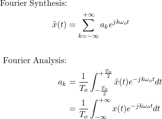
In the previous article we covered how periodic signals can be decomposed into a sum of complex exponentials, the Fourier Series, which led into the concept of Fourier Analysis and Synthesis. Something quite similar can also be achieved for aperiodic signals, where the mathematical equations are known as the Fourier Transform and Inverse Fourier Transform. The main concept behind these more general synthesis and analysis equations is using periodic signals in order to construct aperiodic signals. Any aperiodic signal can be represented by a periodic signal that is shifted and added to itself by multiples of some period T_o. As the period T_o approaches infinity this Fourier series (or linear combination of complex exponentials) is considered a good approximation of the aperiodic signal.

Let's consider an aperiodic signal x(t). A periodic approximation of that signal can be taken as follows:

In other words, a Fourier series is used to represent the periodic x(t), which when the period T_o goes to infinity can represent x(t).

The periodic x(t) can be represented with the Fourier Analysis and Synthesis equations that we covered last time:

Representation using Envelopes

Representing the coefficients of the Fourier series using this representation isn't that useful, which is why envelopes are used. Using envelopes, the Fourier series coefficients can be turned into samples of an envelope. Changing the form of the envelope will allow us to change the shape of the signal over a period, but without being directly dependent on the value of the period. As such, the Fourier series coefficients are expressed as samples of the envelope which are spaced in frequency. Therefore, the Fourier transform, in general, takes us from the Time-Domain to the Frequency-Domain.

The coefficients are defined as:

where T_o a_k = X(ω) when ω = k ω_o, and X(ω) is the envelope of T_o a_k.

Fourier Transform

Using envelopes, the new representation of the Fourier Transform (or analysis equation) is:

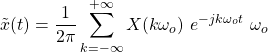
For example the Fourier Transform turns a unit pulse to:

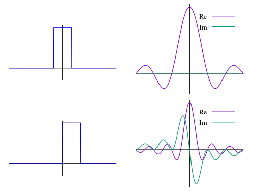
[Image 2]

where the peak of the diagram is the following value:

which is also the value of the previous coefficients, a_k, for ω = k ω_o.

In general, Fourier Series coefficients equal 1/T_o times the samples of the Fourier transform of one period.

As T_o increases the samples taken are more dense, leading us to the representation shown in the diagram.

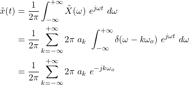
Inverse Fourier Transform

The synthesis part is known as the Inverse Fourier Transform, and mathematically represented as:

In other words, as T_o → ∞:

Fourier Transform of a Periodic Signal

Last, but not least, let's also get into how the Fourier Transform, that was covered today, can be used to represent periodic signals. For the Fourier series, the coefficients are equal to the a_k 's that we already covered. But, when talking about the Fourier Transform new coefficients have to be build, which have to be envelopes of some sort. In other words, a periodic signal x(t) is represented by envelopes, denoted as periodic X(ω).

Let's skip the proof, and just show the equations...

The coefficients, X(ω), and so the analysis part of the Fourier Transform, are given by definition, using the following equation:

As such, the synthesis part, which gives us the periodic signal, is:

RESOURCES:

References

Alan Oppenheim. RES.6-007 Signals and Systems. Spring 2011. Massachusetts Institute of Technology: MIT OpenCourseWare, License: Creative Commons BY-NC-SA.

Images

Mathematical equations used in this article were made using quicklatex.

Block diagrams and other visualizations were made using draw.io

Previous articles of the series

Introduction → Signals, Systems
Signal Basics → Signal Categorization, Basic Signal Types
Signal Operations with Examples → Amplitude and Time Operations, Examples
System Classification with Examples → System Classifications and Properties, Examples
Sinusoidal and Complex Exponential Signals → Sinusoidal and Exponential Signals in Continuous and Discrete Time
LTI System Response and Convolution → Linear System Interconnection (Cascade, Parallel, Feedback), Delayed Impulses, Convolution Sum and Integral
LTI Convolution Properties → Commutative, Associative and Distributive Properties of LTI Convolution
System Representation in Discrete-Time using Difference Equations → Linear Constant-Coefficient Difference Equations, Block Diagram Representation (Direct Form I and II)
System Representation in Continuous-Time using Differential Equations → Linear Constant-Coefficient Differential Equations, Block Diagram Representation (Direct Form I and II)
Continuous-Time Periodic Signals & Fourier Series → Input Decomposition, Fourier Series, Analysis and Synthesis

Final words | Next up

And this is actually it for today's post!

Next time we will get into various useful Properties of the Fourier Transform!

See Ya!

Keep on drifting!

Mathematics - Signals And Systems - Continuous-Time Aperiodic Signals & Fourier Transform